기존에 MobileNet V2 이후로, Efficient Neural Network를 디자인함에 있어서 각 Layer에 Channel Configuration을 FLOPs constraint를 만족하는 것에 우선순위를 두어 Design을 하는 것에 초점을 두었습니다 (i.e., 앞 Layer에서는 Channel을 적게, 뒤 Layer에서는 Channel을 굉장히 많이 사용).
본 논문에서는 각 Layer에서의 Output Feature의 Rank 분석에 기반하여 각 Layer 또는 Block의 Channel 수를 해당 Block의 Index에 Linear하게 Parameterize (i.e, $a*f(i) + b$, 여기서 a와 b는 Learning Parameter) 하는 방법을 제안하였습니다. 여기서 중요한 Motivation은 Layer의 Expressiveness(표현력)이 Output Feature의 Matrix Rank로 표현될 수 있다는 점이고, 사실 이 내용이 현재 연구하고 있는 분야와 관련이 있어 본 논문을 보게 되었습니다. 어떻게 Rank의 Metric을 사용하였는지는 구체적인 언급은 없지만, 아마도 Input에서 Output로 갈 때 Feature Dimesion이 늘어나야 하는 상황에서 Rank가 그만큼 잘 늘어나는지 (?) 정도를 Measure하지 않았을까 추측 합니다.
Rank와 관련된 부분이 사실 이 논문의 핵심은 아니고, 이 논문에서는 Rank를 높이는 방향에서 Intution을 얻어서 각 Layer의 Channel Configuration을 Linear하게 증가하는 방법으로 제안을 하였고 (i.e., 이렇게 하였을때 Rank가 높음을Empirical 하게 보임), Image Classfication, Obejct Detection, 그리고 Image Segmentation 등 다양한 실험에서 좋은 성능을 보여주었습니다. 단순하고 간단한 제안된 방법으로 Channel Configuration 조정만으로도, SOTA NAS 방법들 대비 더 좋은 성능을 보여준 점은 인상 깊은 것 같습니다.
Conference: CVPR 2021
URL: https://arxiv.org/abs/2007.00992
Code: https://github.com/clovaai/rexnet
1. Introduction
Lightweight models shrink some channels for computational efficiency, which leads to promising tradeoffs between computational cost and accuracy. In other words, the degree of channel expansion at layers is quite different, where earlier layers have a smaller channel dimension and deeper layers largely expand above the number of classes. This is to realize flop efficiency by narrow channel dimensions at earlier layers while achieving the model expressiveness with sufficient channel dimension at deeper layers (see Table 1).

This channel configuration for lightweight models became the defacto design convention, but how to adjust the channel dimensions for the optimal under the restricted computational cost has not been profoundly studied. As shown in Table 1, even network architecture search (NAS)-based models were designed upon the convention or little more exploration within few options near the configuration and focused on searching building blocks. Take one step further from the design convention, we hypothesize that the compact models designed by the conventional channel configuration may be limited in the expressive power due to mainly focusing on flop-efficiency; there would exist a more effective configuration over the traditional one.
In this paper, we investigate an effective channel configuration of a lightweight network with additional accuracy gain. Inspired by the works [58, 62], we conjecture the expressiveness of a layer can be estimated by the matrix rank of the output feature. Technically, we study with the averaged rank computed from the output feature of a bunch of networks that are randomly generated with random sizes to reveal the proper range of expansion ratio at an expansion layer and make a link with a rough design principle. Based on the principle, we move forward to find out an overall channel configuration in a network. It turns out that the best channel configuration is parameterized as a linear function by the block index in a network.
2. Expressiveness of a Layer
2.1. Preliminary
Estimating the expressiveness: In language modeling, the authors [58] firstly highlighted that the softmax layer may suffer from turning the logits to the entire class probability due to the rank deficiency. This stems from the low input dimensionality of the final classifier and the vanished nonlinearity at the softmax layer when computing the log probability. The authors proposed a remedy of enhancing the expressiveness, which improved the model accuracy. This implies that a network can be improved by dealing with the lack of expressiveness at certain layers. The authors of [62] compressed a model at layer-level by a low-rank approximation; investigated the amount of compression by computing the singular values of each feature. Inspired by the works, we conjecture that the rank may be closely related to the expressiveness of a network.
*[58] Breaking the softmax bottleneck: A high-rank RNN language model. In ICLR, 2018.
*[62] Efficient and accurate approximations of nonlinear convolutional networks. In CVPR, 2015.
2.2. Empirical Study
Sketch of the study: We aim to study a design guide of a single expansion layer that expands the input dimension. We measure the rank of the output features from the diverse architectures (over 1,000 random-sized networks) and see the trend as varying the input dimensions towards the output dimensions. The rank is originally bounded to the input dimension, but the subsequent nonlinear function will increase the rank above the input dimension [1, 58]. However, a certain network fails to expand the rank close to the output dimension, and the feature will not be fully utilized. We statistically verify the way of avoiding failure when designing the network.
* [1] Low-rank matrix approximation using point-wise operators. IEEE Transactions on Information Theory 2011.
Materials: The networks building blocks consists of 1 ) a single $1 \times 1$ or $3 \times 3$ convolution layer; 2) an inverted bottleneck block with a $3 \times 3$ convolution or $3 \mathrm{x} 3$ depthwise convolution inside. We have the layer output (i.e., feature) $f(\mathbf{W X})$ with $\mathbf{W} \in \mathbb{R}^{d_{\text {out }} \times d_{i n}}$ and the input $\mathbf{X} \in \mathbb{R}^{d_{i n} \times N}$, where $f$ denotes a nonlinear function ${ }^{1}$ with the normalization (we use a BN [25] here). $d_{\text {out }}$ is randomly sampled to realize a random-sized network, and $d_{i n}$ is proportionally adjusted for each channel dimension ratio (i.e., $\left.d_{\text {in }} / d_{\text {out }}\right)$ in the range $[0.1,1.0] . N$ denotes the batch size, where we set $N>d_{\text {out }}>d_{i n}$. We compute rank ratio (i.e., $\left.\operatorname{rank}(f(\mathbf{W} \mathbf{X})) / d_{\text {out }}\right)$ for each model and average them.

Observations: Figure 1 shows how the rank changes with respect to the input channel dimension on average. Dimension ratio ($d_{in}$/$d_{out}$) on the x-axis denotes the reciprocal of the expansion ratio [47]. We observe the followings:
(1) Drastic channel expansion harms the rank. The impact gets bigger with 1) an inverted bottleneck (see Figure 1c); 2) a depthwise convolution (see Figure 1d);
(2) Nonlinearities expand rank. They expand rank more at smaller dimension ratio, and complicated ones such as ELU, or SiLU do more;
(3) Nonlinearities are critical for convolutions. Nonlinearities expand the rank of 1×1 and 3×3 single convolutions more than an inverted bottleneck (see Figure 1a and 1b vs. Figure 1c and 1d).
What we learn from the observations: We learned the followings: 1) an inverted bottleneck is needed to design with the expansion ratio of 6 or smaller values at the first 1×1 convolution; 2) each inverted bottleneck with a depthwise convolution needs a higher channel dimension ratio; 3) a complicated nonlinearity such as ELU and SiLU needs to be placed after 1×1 convolutions or 3×3 convolutions (not depthwise convolutions).
3. Experiment
Our goal is to reveal an effective channel configuration of designing a network under the computational demands. We formulate the following problem:
$\begin{aligned} \max _{c_{i}, i=1 \ldots d} & \operatorname{Acc}\left(N\left(c_{1}, \ldots c_{d}\right)\right) \\ \text { s.t. } \quad & c_{1} \leq c_{2} \leq \cdots \leq c_{d-1} \leq c_{d} \\ & \operatorname{Params}(N) \leq P, \quad \text { FLOPs }(N) \leq F \end{aligned} \quad (1)$
where Acc denotes the top-1 accuracy of the model; ci denotes output channel of i-th block among d building blocks; P and F denote the target parameter size and FLOPs. We search $c_i$ while fixing the network $N$.
3.1. Searching with Channel Parameterization
We represent the channel dimensions at each building block as a piecewise linear function. We parameterize the channel dimensions as $c_i = af(i) + b$, where $a$ and $b$ are to be searched; let f(i) as a piecewise linear function by picking a subset of f(i) up from 1 . . . d. Note that we do not search the building blocks’ expansion ratio. Optimization is done alternatively by searching and training a network. We train each model for 30 epochs for faster training and the early stopping strategy.
3.2. Search Results

We assign four search constraints to aim to search across different target model sizes. After each search, we collect top-10%, middle-10% (i.e., the models between top-50% and 60%), and bottom-10% models in terms of the model accuracy from 200 searched models. To this end, we first visualize the collected models’ channel configuration in Figure 2 of each search; we then report the detailed performance statistics in Table 3.

In Figure 2, we observe that the linear parameterizations by the block index as colored with red enjoy higher accuracies while maintaining similar computational costs. Note that the best models in Table 3 also have the linearly increasing channel configuration. In addition, blue represents the conventional designs for flop efficiency by limiting the channels at earlier layers and giving more channels close to the output. Therefore, we suggest that we need to change the convention (blue) towards the new channel configuration (red).
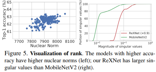
Rank visualization: We study the model expressiveness by analyzing the rank of trained models to see how the linear parameterization affects the rank. We visualize the rank computed from the trained models in two manners; we show the distribution of accuracy vs. rank (represented by the nuclear norm) from 18-depth models; we then compare MobileNetV2 with ReXNet (×0.9) by visualizing the cumulative distribution of the singular values that are normalized to [0, 1] computed from the features of the images in the ImageNet validation set. As shown in Figure 5, we observe 1) a higher-accuracy model has a higher rank; 2) ReXNet clearly expands the rank over the baseline.
3.3. ImageNet Experiment
We train our model on the ImageNet dataset using the standard data augmentation with stochastic gradient descent (SGD) and a minibatch size of 512 on four GPUs. Our model outperforms most of the models searched by NAS including MobileNetV3-Large, MNasNet-A3, MixNet-M, and EfficientNet-B0 (without AutoAug [9]) with at least +0.3pp accuracy improvement. Additionally, we train our model with RandAug to compare it fairly with the other NAS-based models using additional regularization such as Mixup, AutoAug, and RandAug, our model improves all the models including EfficientNetB0 (with AutoAug), FairNas-A, FairDARTS-C, and SE DARTS+ by at least +0.4pp. Strikingly, our model does not require further searches, but it either outperforms or is comparable to NAS-based models.
