최근에 가장 유행하는 One-shot NAS는 Over-parameterized된 Supernet을 학습한 후에, Supernet의 Weight을 재사용하여 (e.g, 추가적인 학습을 하거나 그냥 사용하거나) Resource Constraint를 만족하는 또는 최적의 성능을 내는, Subnet을 찾는 과정을 의미합니다.
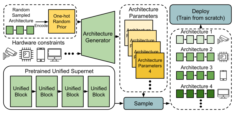
본 논문에서는 기존의 One-shot NAS SOTA 방법들과 성능은 비슷하면서도, 더 적은 Search Cost를 사용하는, 특히 여러개의 Constraint를 만족하는 N개의 모델은 Constant Search Cost로 찾는 방법을 제안하였습니다. 제안된 방법은 크게 1) Architecture Generator를 학습해 Resource Constraint를 만족하는 Architecture Parameter (e.g., 각 Layer에서 어떠한 Configuration을 쓸 것인가)를 Sample하는 방법과 2) Supernet을 구성함에 있어 각 Layer를 구성하는 Unified Block을 제안함으로 Search Efficiency를 높이고 Memory Consumption을 줄일 수 있었습니다. ImageNet에서 H-Swish Activation과 AutoAugment Data Augment를 사용하였을 시, 5 Hour의 Search Cost로 77.1%를 달성하였다고 합니다.
Conference: CVPR 2021
URL: https://arxiv.org/abs/2103.07289
Code: https://github.com/eric8607242/SGNAS
1. Introduction
To improve searching efficiency, one-shot NAS methods were proposed to encode the entire search space into an over-parameterized neural network, called a supernet. Once the supernet is trained, all sub-networks in the supernet can be evaluated by inheriting the weights of the supernet without additional training. One-shot NAS methods can be divided into two categories: differentiable NAS (DNAS) and single-path NAS.
In addition to optimizing the supernet, DNAS utilizes additional differentiable parameters, called architecture parameters, to indicate the architecture distribution in the search space. Because DNAS couples architecture parameters optimization with supernet optimization, for N different hardware constraints, the supernet and the architecture parameters should be trained jointly for N times. In contrast, single-path methods decouple supernet training from architecture searching. For supernet training, only a single path consisting of one block in each layer is activated and is optimized in one iteration. Once the supernet is trained, different search strategies, like the evolution algorithm, can be used to search the architecture under different constraints without retraining the supernet. More flexible than DNAS, yet, re-executing the search strategy for N different constraints is costly and not flexible enough.
In this work, we focus on improving the efficiency and flexibility of the search strategy of the single-path method. The main idea is to search for the best architecture by generating it. First, we decouple supernet training from architecture searching and train the supernet by a single-path method. After obtaining the supernet, we propose to build an architecture generator to generate the best architecture directly. Given a hardware constraint as input, the architecture generator can generate the architecture parameter. When N different constraints are to be met, the search strategy only needs to be conducted once, which is more flexible than N searches required in previous single-path methods.
Training a single-path supernet still requires a lot of GPU memory and time because of the huge number of parameters and complex structure. Previous single-path NAS methods determine a block for each layer, and there may be different candidate blocks with various configurations. Inspired by the fine-grained supernet in AtomNAS, we propose a novel single-path supernet called unified supernet to reduce GPU memory consumption. In the unified supernet, we only construct a block called a unified block in each layer. There are multiple sub-blocks in the unified block, and each sub-block can be implemented by different operations. By combining sub-blocks, all configurations can be described in a block. In this way, the number of parameters of the unified supernet is much fewer than previous single-path methods.
2. Methods
2.1. Architecture Generator
Given the target hardware constraint $C$, the process of the architecture generator can be described as $\boldsymbol{\alpha}=G(C)$ such that $\operatorname{Cost}(\boldsymbol{\alpha})<C$, and we propose the hardware constraint loss $L_C$ as:
$\mathcal{L}_{C}(\boldsymbol{\alpha}, C)=(\operatorname{Cost}(\boldsymbol{\alpha})-C)^{2}$
The cost $\operatorname{Cost}(\boldsymbol{\alpha})$ is differentiable with respect to the architecture parameter $\boldsymbol{\alpha}$, as in DARTs or FBNet. By combining the hardware constraint loss $\mathcal{L}_{C}$ and the cross entropy loss $\mathcal{L}_{val}$, the overall loss of the architecture generator $\mathcal{L}_{G}$ is:
$\mathcal{L}_{G}=\mathcal{L}_{val}\left(\boldsymbol{w}^{*}, \boldsymbol{\alpha}\right)+\lambda \mathcal{L}_{C}(\boldsymbol{\alpha}, C) \quad (10) $
where $\lambda$ is a hyper-parameter to trade-off the validation loss and hardware constraint loss. In practice, we found that the architecture generator easily overfits to a specific hardware constraint. The reason is that it is too difficult to generate complex and high-dimensional architecture parameters based on a given simple integer hardware constraint C.
To address this issue, a prior is given as input to stabilize the architecture generator. We randomly sample a neural architecture from the search space and encode the neural architecture into a one-hot vector to be the prior knowledge of architecture parameters. We name it as a random prior $B=B_{1}, \ldots, B_{L} .$ Formally, $B_{l}=$ one_hot $\left(a_{l}\right), l=1, \ldots, L$, where $a_{l}$ is the $lth$ layer of the neural architecture $a$ randomly sampled from $A$, and $L$ is the total number of layers in the supernet. With the random prior, the architecture generator is to learn the residual from the random prior to the best architecture parameters, and the process of the architecture generator can be reformulated as $\boldsymbol{\alpha}=G(C, B)$ such that $\operatorname{Cost}(\boldsymbol{\alpha})<C$.

Fig. 2 illustrates the architecture of the generator. In each iteration, given the target constraint and the random prior, the architecture generator can generate the architecture parameters $\boldsymbol{\alpha}$. Then, corresponding cost $C_{\boldsymbol{\alpha}}$ can be calculated. We can predict $\hat{y}$ based on the pre-trained supernet $N$ with $\boldsymbol{\alpha}$. The total loss is given by Eqn. (10). Therefore, training the generator is equivalent to searching for the best architectures for various constraints in the proposed SGNAS.
2.2. Unified Supernet
Because inverted bottleneck style basic building block can only represent one configuration with one kernel size and one expansion rate, previous single-path NAS needs to construct blocks of various configurations in each layer, which leads to an exponential increase in parameter numbers and complexity of the supernet. In this work, we propose a unified supernet to improve the efficiency and flexibility of the architecture generator. The only type of block, i.e., unified block, is constructed in each layer. The unified block is built with only the maximum expansion rate $e_{\max }$, i.e., $c_{2}=e_{\max } \times c_{1}$.

Fig. 3 illustrates the idea of a unified block. To make the unified block represent all possible configurations, we replace the depthwise convolution $D$ by $e_{\max }$ sub-blocks, and each sub-block can be implemented by different operations or skip connection. The output tensor of the first pointwise convolution $Y_{1}$ is equally split into $e_{\max }$ parts, $Y_{1,1}, Y_{1,2}, \ldots, Y_{1, e_{\max }} .$ With the sub-blocks $d_{i}$ and split tensors $Y_{1, i}$, we can reformulate depthwise convolution as:
$$
d_{1}\left(Y_{1,1}\right) \circ d_{2}\left(Y_{1,2}\right) \circ \cdots \circ d_{e_{\max }}\left(Y_{1, e_{\max }}\right)
$$
where o denotes the channel concatenation function. With the sub-blocks implemented by different operations, we can simulate blocks with various expansion rates, as shown in Fig. 4. The unified supernet thus can significantly reduce the parameters and GPU memory consumption.

BNs Statistics: As in [28], we suffer from the problem of unstable running statistics of batch normalization (BN). In the unified supernet, because one unified block would represent different expansion rates, the BN scales change more dramatically during training. To address the problem, BN recalibration is used to recalculate the running statistics of BNs by forwarding thousands of training data after training. On the other hand, shadow batch normalization (SBN) [8] or switchable batch normalization [42] are used to stabilize BN. In this work, we utilize SBN to address the large variability issue, as illustrated in Fig. 4. In our setting, there are five different expansion rates, i.e., 2, 3, 4, 5, and 6. We thus take five BNs after the second pointwise convolution block to capture the BN statistics for different expansion rates. With SBN, we can capture different statistics and make supernet training more stable.
Also, the paper introduces some tricks to reduce architecture redundancy (Refer to the paper).
3. Experiments
3.1. ImageNet with SOTAs
This section compares various SOTA one-shot NAS methods that utilize the augmented techniques (e.g., Swish activation function and Squeezeand-Excitation). We directly modify the searched architecture by replacing all ReLU activation with H-Swish activation and equip it with the squeeze-and-excitation module as in AtomNAS. For comparison, similar to the settings in ScarletNAS [9] and GreedyNAS [40], we search architectures under 275M, 320M, and 365M FLOPs, and denote the searched architecture as SGNAS-C, SGNAS-B, and SGNAS-A, respectively. The comparison results are shown in Table 2. The column “Train time” denotes that the time needed to train the supernet, and the column “Search time” denotes that the time needed to search the best architecture based on the pre-trained supernet.

As can be seen, our SGNAS is competitive with SOTAs in terms of top-1 accuracy under different FLOPs. For example, SGNAS-A achieves 77.1% top-1 accuracy. More importantly, SGNAS achieves much higher search efficiency. With the architecture generator and the unified supernet, even for N different architectures under N different hardware constraints, only 5 GPU hours are needed for SGNAS on a Tesla V100 GPU. Supernet retraining is needed for FBNetV2 [36] and AtomNAS [28], which makes the search very inefficient.
3.2. Experiments on NAS-Bench-201
To demonstrate the efficiency and robustness of SGNAS more fairly, we evaluate it based on a NAS benchmark dataset called NAS-Bench-201. Based on the search space defined by NAS-Bench-201, we follow SETN [15] to train the supernet by uniform sampling. After that, the architecture generator is applied to search architectures on the supernet. We search based on the CIFAR-10 dataset and look up the ground-truth performance of the searched architectures on CIFAR-10, CIFAR100, and ImageNet-16-120 datasets, respectively.

We show the 15,625 architectures in NAS-Bench-201 on each dataset as gray dots in Fig. 5 and draw the architectures searched by the architecture generator under different FLOPs as blue rectangles.

