We explore deep reinforcement learning methods for multi-agent domains. We begin by analyzing the difficulty of traditional algorithms in the multi-agent case: Q-learning is challenged by an inherent non-stationarity of the environment, while policy gradient suffers from a variance that increases as the number of agents grows. We then present an adaptation of actor-critic methods that considers action policies of other agents and is able to successfully learn policies that require complex multiagent coordination. Additionally, we introduce a training regimen utilizing an ensemble of policies for each agent that leads to more robust multi-agent policies.
One downside to our approach is that the input space of Q grows linearly (depending on what information is contained in x) with the number of agents N. This could be remedied in practice by, for example, having a modular Q function that only considers agents in a certain neighborhood of a given agent. We leave this investigation to future work.
URL: https://arxiv.org/pdf/1706.02275.pdf
Topic: Multi-Agent RL
Video: https://sites.google.com/site/multiagentac/
Code: https://github.com/openai/multiagent-particle-envs
1. Introduction
There are a number of important applications that involve interaction between multiple agents, where emergent behavior and complexity arise from agents co-evolving together. For example, multi-robot control [21], the discovery of communication and language [31, 8, 25], multiplayer games [28], and the analysis of social dilemmas [17] all operate in a multi-agent domain. Additionally, multi-agent self-play has recently been shown to be a useful training paradigm [29, 32]. Scaling RL to environments with multiple agents is crucial to building artificially intelligent systems that can productively interact with humans and each other.
Unfortunately, traditional reinforcement learning approaches such as Q-Learning or policy gradient are poorly suited to multi-agent environments. One issue is that each agent’s policy is changing as training progresses, and the environment becomes non-stationary from the perspective of any individual agent (in a way that is not explainable by changes in the agent’s own policy). This presents learning stability challenges and prevents the straightforward use of past experience replay, which is crucial for stabilizing deep Q-learning. Policy gradient methods, on the other hand, usually exhibit very high variance when coordination of multiple agents is required. Alternatively, one can use model-based policy optimization which can learn optimal policies via back-propagation, but this requires a (differentiable) model of the world dynamics and assumptions about the interactions between agents. Applying these methods to competitive environments is also challenging from an optimization perspective, as evidenced by the notorious instability of adversarial training methods [11].
In this work, we propose a general-purpose multi-agent learning algorithm that: (1) leads to learned policies that only use local information (i.e. their own observations) at execution time, (2) does not assume a differentiable model of the environment dynamics or any particular structure on the communication method between agents, and (3) is applicable not only to cooperative interaction but to competitive or mixed interaction involving both physical and communicative behavior. The ability to act in mixed cooperative-competitive environments may be critical for intelligent agents; while competitive training provides a natural curriculum for learning [32], agents must also exhibit cooperative behavior (e.g. with humans) at execution time.
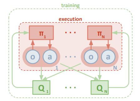
We adopt the framework of centralized training with decentralized execution, allowing the policies to use extra information to ease training, so long as this information is not used at test time. It is unnatural to do this with Q-learning without making additional assumptions about the structure of the environment, as the Q function generally cannot contain different information at training and test time. Thus, we propose a simple extension of actor-critic policy gradient methods where the critic is augmented with extra information about the policies of other agents, while the actor only has access to local information. After training is completed, only the local actors are used at the execution phase, acting in a decentralized manner and equally applicable in cooperative and competitive settings.
Since the centralized critic function explicitly uses the decision-making policies of other agents, we additionally show that agents can learn approximate models of other agents online and effectively use them in their own policy learning procedure. We also introduce a method to improve the stability of multi-agent policies by training agents with an ensemble of policies, thus requiring robust interaction with a variety of collaborator and competitor policies. We empirically show the success of our approach compared to existing methods in cooperative as well as competitive scenarios, where agent populations are able to discover complex physical and communicative coordination strategies.
2. Related Works
3. Background
Markov Games: In this work, we consider a multi agent extension of Markov decision processes (MDPs) called partially observable Markov games [20]. A Markov game for $N$ agents is defined by a set of states $\mathcal{S}$ describing the possible configurations of all agents, a set of actions $\mathcal{A}_{1}, \ldots, \mathcal{A}_{N}$ and a set of observations $\mathcal{O}_{1}, \ldots, \mathcal{O}_{N}$ for each agent. To choose actions, each agent $i$ uses a stochastic policy $\boldsymbol{\pi}_{\theta_{i}}: \mathcal{O}_{i} \times \mathcal{A}_{i} \mapsto[0,1]$, which produces the next state according to the state transition function $\mathcal{T}: \mathcal{S} \times \mathcal{A}_{1} \times \ldots \times \mathcal{A}_{N} \mapsto \mathcal{S} .{ }^{2}$ Each agent $i$ obtains rewards as a function of the state and agent's action $r_{i}: \mathcal{S} \times \mathcal{A}_{i} \mapsto \mathbb{R}$, and receives a private observation correlated with the state $\mathbf{o}_{i}: \mathcal{S} \mapsto \mathcal{O}_{i}$. The initial states are determined by a distribution $\rho: \mathcal{S} \mapsto[0,1]$. Each agent $i$ aims to maximize its own total expected return $R_{i}=\sum_{t=0}^{T} \gamma^{t} r_{i}^{t}$ where $\gamma$ is a discount factor and $T$ is the time horizon.
Q-Learning and Deep Q-Networks (DQN): Q-Learning and DQN [24] are popular methods in reinforcement learning and have been previously applied to multi-agent settings $[8,37] .$ Q-Learning makes use of an action-value function for policy $\boldsymbol{\pi}$ as $Q^{\boldsymbol{\pi}}(s, a)=\mathbb{E}\left[R \mid s^{t}=s, a^{t}=a\right] .$ This $Q$ function can be recursively rewritten as $Q^{\pi}(s, a)=\mathbb{E}_{s^{\prime}}\left[r(s, a)+\gamma \mathbb{E}_{a^{\prime} \sim \pi}\left[Q^{\pi}\left(s^{\prime}, a^{\prime}\right)\right]\right] .$ DQN learns the action-value function $Q^{*}$ corresponding to the optimal policy by minimizing the loss:
$\mathcal{L}(\theta)=\mathbb{E}_{s, a, r, s^{\prime}}\left[\left(Q^{*}(s, a \mid \theta)-y\right)^{2}\right], \quad$ where $\quad y=r+\gamma \max _{a^{\prime}} \bar{Q}^{*}\left(s^{\prime}, a^{\prime}\right) \quad (1)$
where $\bar{Q}$ is a target $\mathrm{Q}$ function whose parameters are periodically updated with the most recent $\theta$, which helps stabilize learning. Another crucial component of stabilizing DQN is the use of an experience replay buffer $\mathcal{D}$ containing tuples $\left(s, a, r, s^{\prime}\right)$. Q-Learning can be directly applied to multi-agent settings by having each agent $i$ learn an independently optimal function $Q_{i}[36] .$ However, because agents are independently updating their policies as learning progresses, the environment appears non-stationary from the view of any one agent, violating Markov assumptions required for convergence of Q-learning. Another difficulty observed in [9] is that the experience replay buffer cannot be used in such a setting since in general, $P\left(s^{\prime} \mid s, a, \boldsymbol{\pi}_{1}, \ldots, \boldsymbol{\pi}_{N}\right) \neq P\left(s^{\prime} \mid s, a, \boldsymbol{\pi}_{1}^{\prime}, \ldots, \boldsymbol{\pi}_{N}^{\prime}\right)$ when any $\boldsymbol{\pi}_{i} \neq \boldsymbol{\pi}_{i}^{\prime}$.
Policy Gradient (PG) Algorithms: Policy gradient methods are another popular choice for a variety of RL tasks. The main idea is to directly adjust the parameters $\theta$ of the policy in order to maximize the objective $J(\theta)=\mathbb{E}_{s \sim p^{\pi}, a \sim \pi_{\theta}}[R]$ by taking steps in the direction of $\nabla_{\theta} J(\theta) .$ Using the Q function defined previously, the gradient of the policy can be written as [34]:
$\nabla_{\theta} J(\theta)=\mathbb{E}_{s \sim p^{\pi}, a \sim \boldsymbol{\pi}_{\theta}}\left[\nabla_{\theta} \log \boldsymbol{\pi}_{\theta}(a \mid s) Q^{\boldsymbol{\pi}}(s, a)\right] \quad (2)$
where $p^{\pi}$ is the state distribution. The policy gradient theorem has given rise to several practical algorithms, which often differ in how they estimate $Q^{\pi}$. For example, one can simply use a sample return $R^{t}=\sum_{i=t}^{T} \gamma^{i-t} r_{i}$, which leads to the REINFORCE algorithm [39]. Alternatively, one could learn an approximation of the true action-value function $Q^{\pi}(s, a)$ by e.g. temporal-difference learning [33]; this $Q^{\pi}(s, a)$ is called the critic and leads to a variety of actor-critic algorithms [33].
Policy gradient methods are known to exhibit high variance gradient estimates. This is exacerbated in multi-agent settings; since an agent’s reward usually depends on the actions of many agents, the reward conditioned only on the agent’s own actions (when the actions of other agents are not considered in the agent’s optimization process) exhibits much more variability, thereby increasing the variance of its gradients.
Deterministic Policy Gradient (DPG) Algorithms. It is also possible to extend the policy gradient framework to deterministic policies $\mu_{\theta}: \mathcal{S} \mapsto \mathcal{A}[30] .$ In particular, under certain conditions we can write the gradient of the objective $J(\theta)=\mathbb{E}_{s \sim p^{\mu}}[R(s, a)]$ as:
$\nabla_{\theta} J(\theta)=\mathbb{E}_{s \sim \mathcal{D}}\left[\left.\nabla_{\theta} \boldsymbol{\mu}_{\theta}(a \mid s) \nabla_{a} Q^{\boldsymbol{\mu}}(s, a)\right|_{a=\boldsymbol{\mu}_{\theta}(s)}\right] \quad (3)$
Since this theorem relies on $\nabla_{a} Q^{\boldsymbol{\mu}}(s, a)$, it requires that the action space $\mathcal{A}$ (and thus the policy $\boldsymbol{\mu}$ ) be continuous. Deep deterministic policy gradient (DDPG) [19] is a variant of DPG where the policy $\boldsymbol{\mu}$ and critic $Q^{\mu}$ are approximated with deep neural networks. DDPG is an off-policy algorithm, and samples trajectories from a replay buffer of experiences that are stored throughout training. DDPG also makes use of a target network, as in DQN [24].
4. Methods

4.1. Multi-Agent Actor-Critic
We would like to operate under the following constraints: (1) the learned policies can only use local information (i.e. their own observations) at execution time, (2) we do not assume a differentiable model of the environment dynamics, unlike in [25], and (3) we do not assume any particular structure on the communication method between agents (that is, we don’t assume a differentiable communication channel). Fulfilling the above desiderata would provide a general-purpose multi-agent learning algorithm that could be applied not just to cooperative games with explicit communication channels, but competitive games. Similarly to [8], we accomplish our goal by adopting the framework of centralized training with decentralized execution. It is unnatural to do this with Q-learning, as the Q function generally cannot contain different information at training and test time. Thus, we propose a simple extension of actor-critic policy gradient methods where the critic is augmented with extra information about the policies of other agents.
More concretely, consider a game with $N$ agents with policies parameterized by $\boldsymbol{\theta}=\left\{\theta_{1}, \ldots, \theta_{N}\right\}$, and let $\boldsymbol{\pi}=\left\{\boldsymbol{\pi}_{1}, \ldots, \boldsymbol{\pi}_{N}\right\}$ be the set of all agent policies. Then we can write the gradient of the expected return for agent $i, J\left(\theta_{i}\right)=\mathbb{E}\left[R_{i}\right]$ as:
$\nabla_{\theta_{i}} J\left(\theta_{i}\right)=\mathbb{E}_{s \sim p^{\boldsymbol{\mu}}, a_{i} \sim \boldsymbol{\pi}_{i}}\left[\nabla_{\theta_{i}} \log \boldsymbol{\pi}_{i}\left(a_{i} \mid o_{i}\right) Q_{i}^{\boldsymbol{\pi}}\left(\mathbf{x}, a_{1}, \ldots, a_{N}\right)\right] \quad (4)$
Here $Q_{i}^{\pi}\left(\mathbf{x}, a_{1}, \ldots, a_{N}\right)$ is a centralized action-value function that takes as input the actions of all agents, $a_{1}, \ldots, a_{N}$, in addition to some state information $\mathrm{x}$, and outputs the Q-value for agent $i$. In the simplest case, $\mathrm{x}$ could consist of the observations of all agents, $\mathrm{x}=\left(o_{1}, \ldots, o_{N}\right)$, however we could also include additional state information if available. Since each $Q_{i}^{\pi}$ is learned separately, agents can have arbitrary reward structures, including conflicting rewards in a competitive setting. We can extend the above idea to work with deterministic policies. If we now consider $N$ continuous policies $\boldsymbol{\mu}_{\theta}$. w.r.t. parameters $\theta_{j}$ (abbreviated as $\boldsymbol{\mu}_{i}$ ), the gradient can be written as:
$\nabla_{\theta_{i}} J\left(\boldsymbol{\mu}_{i}\right)=\mathbb{E}_{\mathbf{x}, a \sim \mathcal{D}}\left[\left.\nabla_{\theta_{i}} \boldsymbol{\mu}_{i}\left(a_{i} \mid o_{i}\right) \nabla_{a_{i}} Q_{i}^{\boldsymbol{\mu}}\left(\mathbf{x}, a_{1}, \ldots, a_{N}\right)\right|_{a_{i}=\boldsymbol{\mu}_{i}\left(o_{i}\right)}\right] \quad (5)$
Here the experience replay buffer $\mathcal{D}$ contains the tuples $\left(\mathbf{x}, \mathbf{x}^{\prime}, a_{1}, \ldots, a_{N}, r_{1}, \ldots, r_{N}\right)$, recording experiences of all agents. The centralized action-value function $Q_{i}^{\boldsymbol{\mu}}$ is updated as:
$\mathcal{L}\left(\theta_{i}\right)=\mathbb{E}_{\mathbf{x}, a, r, \mathbf{x}^{\prime}}\left[\left(Q_{i}^{\mu}\left(\mathbf{x}, a_{1}, \ldots, a_{N}\right)-y\right)^{2}\right], \quad y=r_{i}+\left.\gamma Q_{i}^{\boldsymbol{\mu}^{\prime}}\left(\mathbf{x}^{\prime}, a_{1}^{\prime}, \ldots, a_{N}^{\prime}\right)\right|_{a_{j}^{\prime}=\boldsymbol{\mu}_{j}^{\prime}\left(o_{j}\right)} \quad (6)$
where $\boldsymbol{\mu}^{\prime}=\left\{\boldsymbol{\mu}_{\theta_{1}^{\prime}}, \ldots, \boldsymbol{\mu}_{\theta_{N}^{\prime}}\right\}$ is the set of target policies with delayed parameters $\theta_{i}^{\prime} .$ As shown in Section 5, we find the centralized critic with deterministic policies works very well in practice, and refer to it as multi-agent deep deterministic policy gradient (MADDPG). We provide the description of the full algorithm in the Appendix.
A primary motivation behind MADDPG is that, if we know the actions taken by all agents, the environment is stationary even as the policies change, since $P\left(s^{\prime} \mid s, a_{1}, \ldots, a_{N}, \boldsymbol{\pi}_{1}, \ldots, \boldsymbol{\pi}_{N}\right)=$ $P\left(s^{\prime} \mid s, a_{1}, \ldots, a_{N}\right)=P\left(s^{\prime} \mid s, a_{1}, \ldots, a_{N}, \boldsymbol{\pi}_{1}^{\prime}, \ldots, \boldsymbol{\pi}_{N}^{\prime}\right)$ for any $\boldsymbol{\pi}_{i} \neq \boldsymbol{\pi}_{i}^{\prime} .$ This is not the case if we do not explicitly condition on the actions of other agents, as done for most traditional RL methods.
Note that we require the policies of other agents to apply an update in Eq. 6. Knowing the observations and policies of other agents is not a particularly restrictive assumption; if our goal is to train agents to exhibit complex communicative behavior in simulation, this information is often available to all agents. However, we can relax this assumption if necessary by learning the policies of other agents from observations — we describe a method of doing this in Section 4.2.
4.2. Inferring Policies of Other Agents
To remove the assumption of knowing other agents' policies, as required in Eq. 6 , each agent can additionally maintain an approximation $\hat{\mu}_{\phi^{j}}$ (where $\phi$ are the parameters of the approximation; henceforth $\hat{\boldsymbol{\mu}}_{i}^{J}$ ) to the true policy of agent $j, \boldsymbol{\mu}_{j}$. This approximate policy is learned by maximizing the log probability of agent $j$ 's actions, with an entropy regularize:
$\mathcal{L}\left(\phi_{i}^{j}\right)=-\mathbb{E}_{o_{j}, a_{j}}\left[\log \hat{\boldsymbol{\mu}}_{i}^{j}\left(a_{j} \mid o_{j}\right)+\lambda H\left(\hat{\boldsymbol{\mu}}_{i}^{j}\right)\right] \quad (7)$
where $H$ is the entropy of the policy distribution. With the approximate policies, $y$ in Eq. 6 can be replaced by an approximate value $\hat{y}$ calculated as follows:
$\hat{y}=r_{i}+\gamma Q_{i}^{\boldsymbol{\mu}^{\prime}}\left(\mathbf{x}^{\prime}, \hat{\boldsymbol{\mu}}_{i}^{\prime 1}\left(o_{1}\right), \ldots, \boldsymbol{\mu}_{i}^{\prime}\left(o_{i}\right), \ldots, \hat{\boldsymbol{\mu}}_{i}^{\prime N}\left(o_{N}\right)\right) \quad (8)$
where $\hat{\mu}_{i}^{\prime j}$ denotes the target network for the approximate policy $\hat{\boldsymbol{\mu}}_{i}^{j}$. Note that Eq. 7 can be optimized in a completely online fashion: before updating $Q_{i}^{\boldsymbol{\mu}}$, the centralized Q function, we take the latest samples of each agent $j$ from the replay buffer to perform a single gradient step to update $\phi_{i}^{j} .$ Note also that, in the above equation, we input the action log probabilities of each agent directly into $Q$, rather than sampling.
4.3. Agents with Policy Ensembles
As previously mentioned, a recurring problem in multi-agent reinforcement learning is the environment's non-stationarity due to the agents’ changing policies. This is particularly true in competitive settings, where agents can derive a strong policy by overfitting to the behavior of their competitors. Such policies are undesirable as they are brittle and may fail when the competitors alter strategies. To obtain multi-agent policies that are more robust to changes in the policy of competing agents, we propose to train a collection of $K$ different sub-policies. At each episode, we randomly select one particular sub-policy for each agent to execute. Suppose that policy $\boldsymbol{\mu}_{i}$ is an ensemble of $K$ different sub-policies with sub-policy $k$ denoted by $\boldsymbol{\mu}_{\theta_{i}^{(k)}}$ (denoted as $\left.\boldsymbol{\mu}_{i}^{(k)}\right)$. For agent $i$, we are then maximizing the ensemble objective: $J_{e}\left(\boldsymbol{\mu}_{i}\right)=\mathbb{E}_{k \sim \operatorname{unif}(1, K), s \sim p^{\mu}, a \sim \boldsymbol{\mu}_{i}^{(k)}}\left[R_{i}(s, a)\right] .$
Since different sub-policies will be executed in different episodes, we maintain a replay buffer $\mathcal{D}_{i}^{(k)}$ for each sub-policy $\boldsymbol{\mu}_{i}^{(k)}$ of agent $i$. Accordingly, we can derive the gradient of the ensemble objective with respect to $\theta_{i}^{(k)}$ as follows:
$\nabla_{\theta_{i}^{(k)}} J_{e}\left(\boldsymbol{\mu}_{i}\right)=\frac{1}{K} \mathbb{E}_{\mathbf{x}, a \sim \mathcal{D}_{i}^{(k)}}\left[\left.\nabla_{\theta_{i}^{(k)}} \boldsymbol{\mu}_{i}^{(k)}\left(a_{i} \mid o_{i}\right) \nabla_{a_{i}} Q^{\boldsymbol{\mu}_{i}}\left(\mathbf{x}, a_{1}, \ldots, a_{N}\right)\right|_{a_{i}=\boldsymbol{\mu}_{i}^{(k)}\left(o_{i}\right)}\right] \quad (9)$
5. Experiments
5.1. Environments
To perform our experiments, we adopt the grounded communication environment proposed in [25] $^{3}$, which consists of $N$ agents and $L$ landmarks inhabiting a two-dimensional world with continuous space and discrete-time. Agents may take physical actions in the environment and communication actions that get broadcasted to other agents. Unlike [25], we do not assume that all agents have identical action and observation spaces, or act according to the same policy $\pi .$ We also consider games that are both cooperative (all agents must maximize a shared return) and competitive (agents have conflicting goals). Some environments require explicit communication between agents in order to achieve the best reward, while in other environments agents can only perform physical actions. We provide details for each environment below.

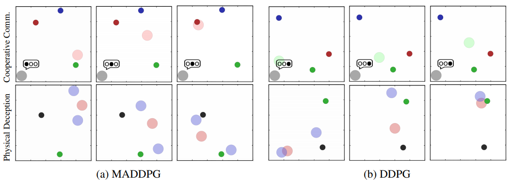
Cooperative communication: This task consists of two cooperative agents, a speaker and a listener, who are placed in an environment with three landmarks of differing colors. At each episode, the listener must navigate to a landmark of a particular color and obtains a reward based on its distance to the correct landmark. However, while the listener can observe the relative position and color of the landmarks, it does not know which landmark it must navigate to. Conversely, the speaker’s observation consists of the correct landmark color, and it can produce a communication output at each time step which is observed by the listener. Thus, the speaker must learn to output the landmark color based on the motions of the listener. Although this problem is relatively simple, as we show in Section 5.2 it poses a significant challenge to traditional RL algorithms.
Predator-prey: In this variant of the classic predator-prey game, N slower cooperating agents must chase the faster adversary around a randomly generated environment with L large landmarks impeding the way. Each time the cooperative agents collide with an adversary, the agents are rewarded while the adversary is penalized. Agents observe the relative positions and velocities of the agents and the positions of the landmarks.
Cooperative navigation: In this environment, agents must cooperate through physical actions to reach a set of L landmarks. Agents observe the relative positions of other agents and landmarks and are collectively rewarded based on the proximity of any agent to each landmark. In other words, the agents have to ‘cover’ all of the landmarks. Further, the agents occupy significant physical space and are penalized when colliding with each other. Our agents learn to infer the landmark they must cover, and move there while avoiding other agents.
Physical deception: Here, N agents cooperate to reach a single target landmark from a total of N landmarks. They are rewarded based on the minimum distance of any agent to the target (so only one agent needs to reach the target landmark). However, the alone adversary also desires to reach the target landmark; the catch is that the adversary does not know which of the landmarks is the correct one. Thus the cooperating agents, who are penalized based on the adversary's distance to the target, learn to spread out and cover all landmarks so as to deceive the adversary.
5.2. Comparison to Decentralized Reinforcement Learning Methods
Unless otherwise specified, our policies are parameterized by a two-layer ReLU MLP with 64 units per layer. The messages sent between agents are soft approximations to discrete messages, calculated using the GumbelSoftmax estimator [14]. To evaluate the quality of policies learned in competitive settings, we pitch MADDPG agents against DDPG agents and compare the resulting success of the agents and adversaries in the environment. We train our models until convergence and then evaluate them by averaging various metrics for 1000 further iterations.
We first examine the cooperative communication scenario. Despite the simplicity of the task (the speaker only needs to learn to output its observation), traditional RL methods such as DQN, Actor-Critic, the first-order implementation of TRPO, and DDPG all fail to learn the correct behavior (measured by whether the listener is within a short distance from the target landmark). In practice, we observed that the listener learns to ignore the speaker and simply moves to the middle of all observed landmarks. We plot the learning curves over 25000 episodes for various approaches in Figure 4.
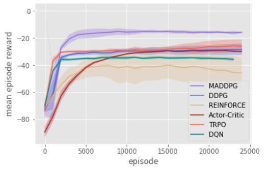
We hypothesize that a primary reason for the failure of traditional RL methods in this (and other) multi-agent settings is the lack of a consistent gradient signal. For example, if the speaker utters the correct symbol while the listener moves in the wrong direction, the speaker is penalized. This problem is exacerbated as the number of time steps grows: we observed that traditional policy gradient methods can learn when the objective of the listener is simply to reconstruct the observation of the speaker in a single time step, or if the initial positions of agents and landmarks are fixed and evenly distributed. This indicates that many of the multi-agent methods previously proposed for scenarios with short time horizons (e.g. [16]) may not generalize to more complex tasks. Conversely, MADDPG agents can learn coordinated behavior more easily via the centralized critic. In the cooperative communication environment, MADDPG is able to reliably learn the correct listener and speaker policies, and the listener is often (84.0% of the time) able to navigate to the target.
A similar situation arises for the physical deception task: when the cooperating agents are trained with MADDPG, they are able to successfully deceive the adversary by covering all of the landmarks around 94% of the time when L = 2 (Figure 5). Furthermore, the adversary success is quite low, especially when the adversary is trained with DDPG (16.4% when L = 2). This contrasts sharply with the behavior learned by the cooperating DDPG agents, who are unable to deceive MADDPG adversaries in any scenario and do not even deceive other DDPG agents when L = 4.
5.3. Effect of Learning Policies of Other Agents
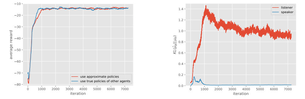
We evaluate the effectiveness of learning the policies of other agents in the cooperative communication environment, following the same hyperparameters as the previous experiments and setting λ = 0.001 in Eq. 7. The results are shown in Figure 7. We observe that despite not fitting the policies of other agents perfectly (in particular, the approximate listener policy learned by the speaker has a fairly large KL divergence to the true policy), learning with approximated policies is able to achieve the same success rate as using the true policy, without a significant slowdown in convergence.
5.4. Effect of Training with Policy Ensembles
We focus on the effectiveness of policy ensembles in competitive environments, including keep-away, cooperative navigation, and predator-prey. We choose K = 3 sub-policies for the keep-away and cooperative navigation environments, and K = 2 for predator-prey. To improve convergence speed, we enforce that the cooperative agents should have the same policies at each episode, and similarly for the adversaries. To evaluate the approach, we measure the performance of ensemble policies and single policies in the roles of both agent and adversary. The results are shown on the right side of Figure 3. We observe that agents with policy ensembles are stronger than those with a single policy. In particular, when pitting ensemble agents against single policy adversaries (second to left bar cluster), the ensemble agents outperform the adversaries by a large margin compared to when the roles are reversed (third to left bar cluster).


